Performing accurate simulation of turbulent flows is still a challenging topic today, especially with limited computational resources. Although the Navier-Stokes equations are perfectly valid in the turbulent flow regime, one typically have to resort to some form of turbulence modeling in order to reduce computational costs, whereby small scale flow fluctuations are effectively filtered out and subsequently approximated by the turbulence model.
The most commonly used turbulence models are currently two equation models, typically the k-epsilon and k-omega models (available with the OpenFOAM CFD solver interface, and large eddy simulation (LES) models. These models typically introduce several additional non-linear equations and may still require very high resolution in both time and space. For simple flow cases and geometries one can instead use an algebraic turbulence model (also called zero-equation model), which greatly simplifies the equations and reduces CFD simulation costs.
Custom definition and implementation of an algebraic turbulence model in FEATool Multiphysics is discussed in the following. In particular, the simple equation expression and coefficient syntax highlights how the turbulence model easily can be defined in FEATool.
Algebraic Turbulence Model Definition
The algebraic turbulence model introduced here is based on Prandtl’s mixing length theory, and works by introducing an additional turbulent viscosity in regions where velocity fluctuations are expected to be high [1]. That is
\[ \mu_{E}(\mathbf{x}) = \mu_F + \mu_T(\mathbf{x}) \]
where the total or effective viscosity $\mu_{E}$ is the sum of the viscosity of the fluid $\mu_F$ and the turbulent viscosity $\mu_T$. This lowers the local Reynolds number allowing the equations to converge.
By using dimensional analysis the kinematic turbulent viscosity must be the product of a velocity scale and a length scale. Moreover, assuming that the small scale turbulent velocity fluctuations (Reynolds stresses) to be modeled can be related to the mean velocity, then we have that the turbulent viscosity can be expressed as
\[ \mu_T(\mathbf{x}) = \rho\ l_{mix}(\mathbf{x})^2|\nabla u| \]
where the mixing length $l_{mix}$ represents the average length a turbulent fluid packet and eddy can travel before breaking up. This can be modeled as the minimum of the shortest distance to the walls, and a characteristic length $l_c$, that is
\[ l_{mix} = min(\kappa\ l_{wall}, Const\ l_c) \]
where $\kappa = 0.41$ is the von Karman constant. This model assumption works well for simple two-dimensional flows such as for example in wakes, jets, and mixing, shear, and boundary layers. Modeling constants and characteristic lengths for these types of flow regimes have been determined empirically, and are given in the table below [2]
| Flow type | $Const$ | $l_c$ |
|---|---|---|
| Mixing layer | 0.07 | Layer width |
| Jet | 0.09 | Jet half-width |
| Wake | 0.16 | Wake half-width |
| Axisymmetric jet | 0.075 | Jet half-width |
| Boundary layer (outer) | 0.09 | Boundary layer thickness |
Note that this model is not really accurate or recommended for complex flows such as those involving separation and/or recirculation.
Algebraic Turbulence Model Implementation
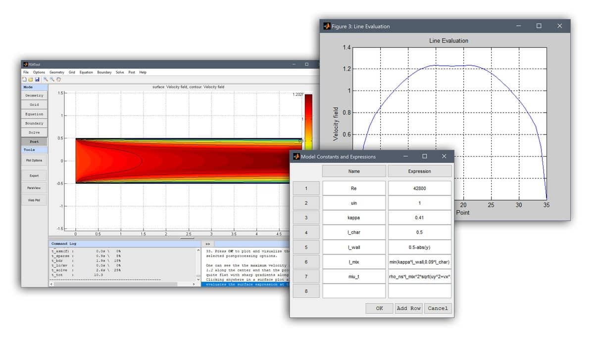
The model described above is used in the following turbulent channel
flow problem with Reynolds number, Re = 42800. Since the channel
geometry is defined as a rectangle with height 1 and width 5
length units, the wall and characteristic lengths are easy to
define. The distance to the walls can simply be computed as
0.5-abs(y) with the characteristic length taken as the maximum wall
distance $l_c = max(l_{wall})$, which here will be a constant value
of 0.5.

The turbulent viscosity can now simply be formulated by using the
constants and expressions given from table below. Note that FEATool
Multiphysics does not require you to do any programming, but allows
you to enter equation and boundary variables, and expressions just as
you would write them on paper. This includes using mathematical
operators (such as min, max, and abs), space coordinates (for
example x and y), and evaluation dependent variables and their
derivatives (here uy and vx). See the post on
modeling with non-constant coefficients in FEATool Multiphysics for more information about valid expression syntax.
| Name | Expression |
|---|---|
kappa | 0.41 |
l_char | 0.5 |
l_wall | 0.5-abs(y) |
l_mix | min(kappa*l_wall,0.09*l_char) |
miu_t | rho_ns*l_mix^2*sqrt(uy^2+vx^2) |
The effective viscosity expression could technically be entered just
as it is, but it is in practice often preferable to enter the
different factors in the Model Coefficients and Expressions box and
simply use miu_t where ever the turbulent viscosity is referred
to. This also makes it easier to later go back and modify or change
the model.
Detailed step-by-step instructions how to implement the turbulence model in this example can be found in the linked tutorial below. (Note that the mentioned built-in turbulence model GUI options in step 13 will be available with the FEATool version 1.12 and later, the manual implementation proceeds from step 41 onwards.)
Alternatively, a FEATool step-by-step tutorials model model can be
started by selecting Model Examples and Tutorials… > Fluid
Dynamics > Turbulent Channel Flow from the File menu in the
FEATool Multiphysics GUI.
References
[1] Versteeg HK, Malalasekera W. An Introduction to Computational Fluid Dynamics: The Finite Volume Method. Longman Scientific and Technical, England, 1995.
[2] Rodi W. Turbulence Models and their Application in Hydraulics, IAHR, Netherlands, June, 1980.