FEATool Multiphysics has been designed to be as easy to use as possible, and conveniently features built-in parsing and evaluation of non-constant variables and coefficients. This allows users to quickly and easily enter modeling expressions formulated much as one would write on paper, all without having to develop, write, and compile external user defined functions as other more complex simulation software often requires.
The following applies to all physics coefficients such as point
constraints, boundary conditions, equation coefficients, initial
conditions and postprocessing expressions, as well as command line
functions such as evalexpr,
intsubd,
intbdr,
minmaxsubd,
minmaxbdr, and
postplot. A coefficient may be
composed as a string expression including any number of the various
coefficient types listed below, combined with the operators
+-*/^, parentheses pairs (), as well as
numeric constants and scalars.
Space coordinates
The space coordinates x, y, and
z for Cartesian coordinate systems, and r
and z for axi-symmetric and cylindrical coordinate
systems are valid coefficient expressions. (Note that the space
coordinate names can be re-assigned from their default definitions
when starting a New Model).
The y-coordinate is for example used to define a parabolic velocity
inlet profile as uinlet =
4*0.3/0.41^2*y*(0.41-y) in the flow around a
cylinder CFD tutorial example.
Dependent variables
Solution unknowns or dependent variables can also be used in
coefficients, with their corresponding names given by the included
physics modes, such as for example T for temperature. (As
with the space coordinate names, dependent variable names may also be
re-defined from the default names when a new physics mode is
added. Also note that adding dependent variables in coefficients often
make a problem more non-linear and harder to solve.)
The introductory
heat transfer multiphysics model for
example shows how the temperature T is coupled to the
fluid flow via the source term
alpha*g*rho*(T-Tc), where alpha, g, rho,
and Tc, are model constants, while the flow velocities
u and v in turn are coupled back and driving
the temperature field through the convective terms.
Space derivatives of dependent variables
By appending a space coordinate postfix to a dependent variable, for
example Tx, the derivatives in the corresponding
direction can be evaluated (in the example here Tx is equivalent to
$\frac{\partial T}{\partial x}$). The capacitance in the
spherical capacitor model tutorial
is for example calculated by integrating the expression
eps0*epsr*(Vr^2+Vz^2)*pi*r, where V is
the computed potential.
Second order derivatives, as for example Txy equivalent
to $\frac{\partial T}{\partial x\partial y}$, can also be evaluated
for dependent variables discretized by the second order Lagrange
finite element basis functions.
Note that derivatives of dependent variables are evaluated by direct differentiation of the underlying FEM shape function polynomials and some overall accuracy may be lost in this process. For example, a variable discretized with a first order linear basis function, will feature a piecewise constant first derivative on each element, and zero second derivative (even if a global second derivative would exist analytically). For higher order accuracy with derivatives a projection or gradient reconstruction technique is necessary.
Time
The variable name t is reserved for the current time in
instationary simulations (evaluates to 0 for stationary
problems). For example, the
instationary flow around a cylinder example
defines a parabolic and time dependent inlet velocity as
uinlet =
6*sin(pi*t/8)*(y*(0.41-y))/0.41^2.
Normals
Boundary coefficients may use the external normals by prefixing a
space dimension name with the character n, as for example
nx for the normal in the x-direction. Boundary normals
are evaluated and computed as the outward pointing unit vector from
the center of each external cell edge or face.
Discontinuous functions
Logical switch expressions such as T>0 and
T<=T0 are also valid syntax and will evaluate to 1 when
true and 0 everywhere else. Valid expressions may include the
characters <, >, <=,
>=, &, and | (corresponding to
the less than, greater than, less than or equal, greater than
or equal, and, and or operators).
These types of switch expressions can be used to build quite complex
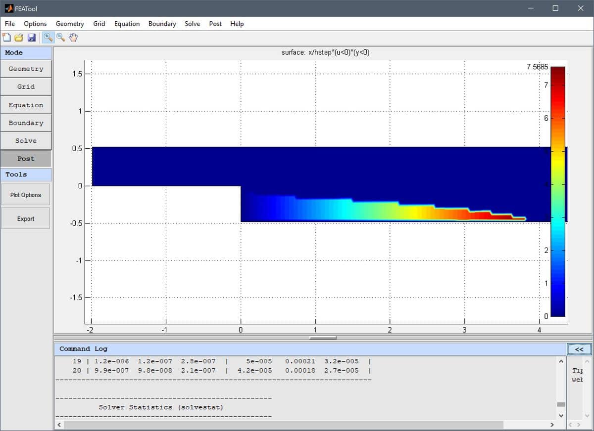
expressions and coefficients, for example in the
flow over a backwards facing step model
the recirculation region is highlighted and visualized with the
postprocessing expression
x/hstep*(u<0)*(y<0). This expression
effectively isolates the region in y < 0 where the x-velocity u is
negative, and overlays it with the scaled coordinate x/hstep,
resulting in the following plot

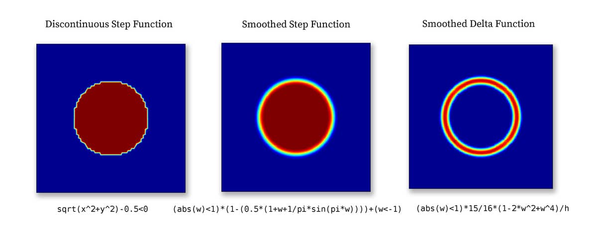
Abruptly varying and discontinuous functions like these can sometimes introduce numerical instabilities if used in equation and boundary conditions. From the perspective of the solver it might then be preferable to use a regularized or smoothed Heaviside function, such as
(abs(w)<1)*(1-(0.5*(1+w+1/pi*sin(pi*w)))) + (w<-1)
or a smoothed Dirac delta function
(w>-1 & w<1)*15/16*(1-2*w^2+w^4)/h_grid
where w is a weighting function defining the transition and width of
the smoothed region. For example, with w =
(sqrt(x^2+y^2)-0.5)/(2h_grid) a circle with radius 0.5
and transition region width 2h_grid is defined as shown below.

Smoothed step and delta functions are commonly used in models with moving and immersed boundaries which cannot be resolved by the mesh. Step functions are used to define the discontinuous materials, and delta functions to define surface tension forces and reactions. For example see the multiphase flow models ex_multiphase1.
Built-in functions
All of the common built-in
mathematical functions and constants in MATLAB,
such as pi, eps, sqrt,
sin, cos, log,
exp, abs etc., may also be used to compose
expressions.
Tabulated and Interpolated Data
In cases where coefficients are to be interpolated from tabulated data, it is possible to use the finterpn function. In this case the data must be available as space (txt) or comma separated (CSV) ASCII text files, where each column represents data points or values (last column), for example a 3-dimensional interpolation table could look like the following (with 2x3xN interpolation points in the x, y, and z-directions ordered according to ndgrid, respectively)
  x1, y1, z1, v1
  x2, y1, z1, v2
  x1, y2, z1, v3
  x2, y2, z1, v4
  x1, y3, z1, v5
  x2, y3, z1, v6
        ...
  x1, y1, zN, vM-5
        ...
  x2, y3, zN, vM
or alternatively a binary MATLAB .mat file with corresponding data. Tabulated equation and boundary coefficients can for example then be specified as
finterpn('C:\path_to\my_tabulated_data.csv',x,T)
where here the full path of the data file is here given as
‘C:\path_to\my_tabulated_data.csv’ (note the single
quotes to specify a string), and interpolation is performed for both
x coordinates and the dependent variable T.
A simple heat transfer tutorial example, featuring tabulated the coefficient of heat conductivity (as a function of Temperature) is available in the tutorials section.
For more complex coefficients a custom user-defined function can be used as described below.
Custom and user-defined functions
If a combination of the above methods is insufficient to implement an expression, or the expression can not be described analytically one can use a custom MATLAB m-file function when using the toolbox with MATLAB (currently not as a stand-alone app).
This could be the case if one wants to use tabulated or experimental data as input which must be interpolated, or complex coefficients with memory effects such as hysteresis.
Please see the corresponding section on custom and user-defined functions in the FEATool Multiphysics documentation for more details .
Reserved coefficient names
The coefficient name h_grid is reserved for the mean grid
cell size or diameter, and is primarily used in the artificial and
convective stabilization techniques.
Internal and local variables may be prefixed with double underscores
__varname, and it is therefore not recommended to name
variables with underscores to prevent potential name collisions.
Tips
An easy way to test and check an expression for correctness is to simply plot and visualize it in postprocessing mode.
For two-dimensional surface plots in the FEATool GUI one can simply click on a point in the plot to evaluate the visualized expression in the point.
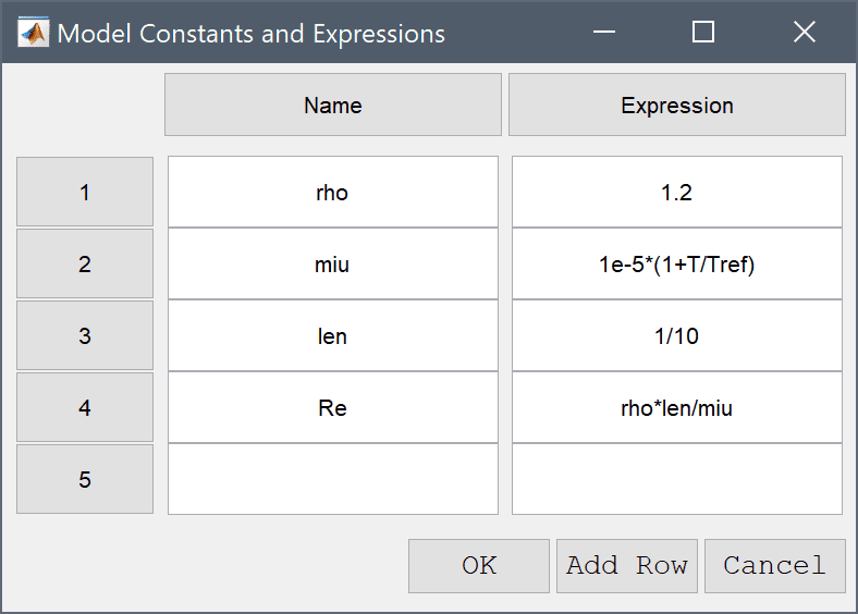
When working in the FEATool GUI it is often convenient to use the Model Constants and Expressions dialog box to define and store modeling expressions. The named expressions are then available everywhere in the GUI from equation coefficients to postprocessing expressions.

The more non-linearities that are introduced the harder it will be for the solver to converge to a solution. Highly non-linear problems typically require more relaxation (which can be achieved by decreasing the Non-linear relaxation parameter in the Solver Settings) and a very good initial guess. One can try to introduce a scalar weighting coefficient to the non-linear coefficients, and step by step increasing it from 0 (no contributions) to 1 (fully non-linear contributions) while using the previous solution as initial guess. Lastly, for stationary problems one can also employ pseudo time stepping with the Backward-Euler scheme to try to use the time dependent solver to reach a steady state.