Axisymmetric Stress-Strain Script Modeling

Continuing on the previous post on axisymmetric modeling in FEATool, we will here take a look at how to model axisymmetric stress-strain from structural mechanics by entering and parsing the governing equations directly into FEATool using MATLAB m-file scripting. The problem we will be looking at is a hollow sphere with is affected by a high uniform pressure from the inside. (Although this tutorial uses the MATLAB m-script and custom equation approach to set up and run the model, the FEATool GUI with predefined axisymmetric physics modes can be used as well.)

First is to define the fea struct which will contain all modeling and problem data. The space dimension coordinate names are chosen as r and z, and their corresponding displacements as u and w. In this case linear Lagrange finite element shape functions sflag1 are used for the FEM discretization.

fea.sdim = { 'r' 'z' };
fea.dvar = { 'u' 'w' };
fea.sfun = { 'sflag1' 'sflag1' };

Next, is to create the computational geometry and grid. By using axisymmetry we are able to save a lot of computational cost by reducing the geometry from three to two dimensions. Since we are looking at a perfect symmetric spherical sphere or shell we can also get away with only modeling a single quadrant of a ring. Such a grid can be created with the help of the ringgrid function, as follows

r_i = 1;
r_o = 2;
fea.grid = ringgrid( 12, 72, r_i, r_o );
fea.grid = delcells( fea.grid, selcells( fea.grid, '(x<=eps) + (y<=eps)') );

The derivation of the axisymmetric stress strain equations is left to the reader, but they are defined in two string equation variables for the radial r and z-directions, respectively. The equations are also parsed by parseeqn to generate the weak FEM formulation stored in the fea.eqn struct.

eqn_r = '- c1*( (1-nu)*ur_r + nu*wz_r + nu/r*( u_r - ur_t - wz_t ) - (1-nu)/r^2*u_t ) - c1*c2*( uz_z + wr_z ) = 2*pi*r*Fr';
eqn_z = '- c1*( nu*ur_z + nu/r*u_z + (1-nu)*wz_z ) - c1*c2*( uz_r + wr_r ) = 2*pi*r*Fz';
fea.eqn  = parseeqn( { eqn_r eqn_z }, fea.dvar, fea.sdim );

Furthermore, equation coefficients and constants are defined in the fea.expr field. The empty cells are simply placeholders for coefficient string descriptions and names used by the FEATool GUI, and not needed here

nu = 0.3;
E  = 200e9;
c1 = E / ((1+nu)*(1-2*nu) );
c2 = (1-2*nu) / 2;
fea.expr = { 'c1' [] [] {[num2str(c1*2*pi),'*r']} ;
             'c2' [] [] {c2} ;
             'nu' [] [] {nu} ;
             'Fr' [] [] {0} ;
             'Fz' [] [] {0} };

Boundary conditions must also be prescribed. In this case a force acting in the normal direction of the inner boundary (number 1), and also zero normal displacements on the symmetry boundaries (3 and 4). (Note that one can use the plotbdr function to visualize and see the boundary numbering).

p = 20e4;
fea.bdr.d = { [] [] []  [0] ;
              [] [] [0] []  };
fea.bdr.n = { [num2str(p*2*pi),'*r*-nr'] [] [] [] ;
              [num2str(p*2*pi),'*r*-nz'] [] [] [] };

Lastly the whole fea problem struct is checked and parsed and sent to the static solver.

fea       = parseprob( fea );
fea.sol.u = solvestat( fea );

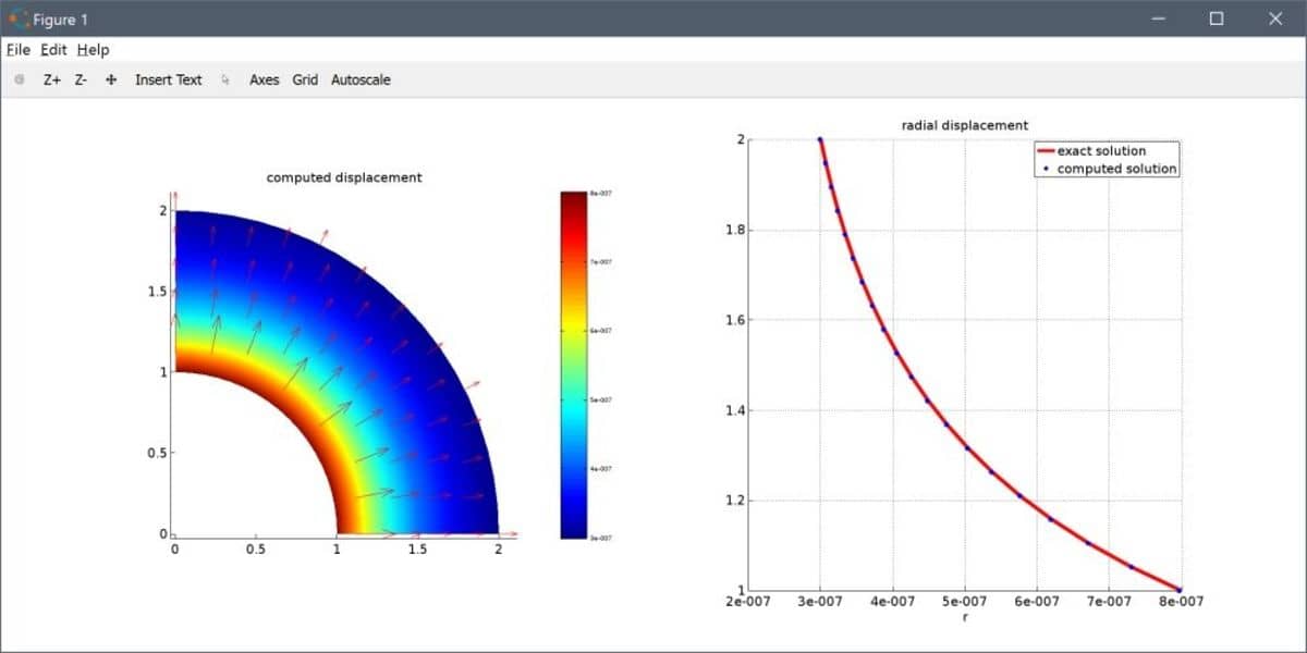
The solution can be visualized, plotted, and compared to the expected analytical displacement of a hollow sphere.

n = 20;
r = linspace(r_i,r_o,n);
z = zeros(1,n);
u_ref = 1./(2*E*(r_o^3-r_i^3)*r.^2) .* (2*(p*r_i^3)*(1-2*nu)*r.^3+p*(1+nu)*r_o^3*r_i^3);
u = evalexpr( 'u', [r;z], fea );

subplot(1,2,1)
postplot( fea, 'surfexpr', 'sqrt(u^2+w^2)', 'arrowexpr', {'u' 'w'} )
title('computed displacement')
subplot(1,2,2), hold on
plot(u_ref,r,'r-')
plot(u,r,'b.')
title( 'radial displacement')
legend('exact solution','computed solution')
xlabel('r')
grid on

The complete FEATool m-script file is available for download from the link below together with a selection of other axisymmetric stress strain benchmark examples.